Univariate Analysis

Data Summary and Histogram

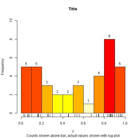
summary(Y) # display data summary stem(Y) # visualise the distribution with a stem-and-leaf plot hist(Y) # visualise the distribution with histogram rug(Y) # to show actual observations

Boxplot

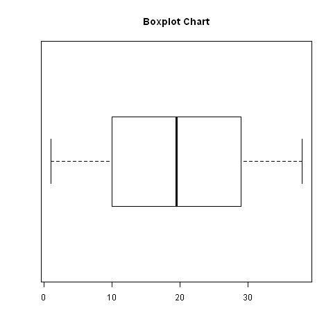
boxplot(X, notch=F, horizontal=T, main="Boxplot Chart") # display the distribution as a Boxplot

Compare Histograms With Different Numbers of Observations

qqnorm(X, main="QQ plot vs Normal distribution", ylab = "X") # display normal QQ plot qqline(X, col=3) # display QQ line

Display A Histogram With The Actual Counts

h <- hist(Y, breaks=seq(0, 1, by=0.1), plot=F) #1 str(h) #2 plot(h, col=heat.colors(length(h$mids))[length(h$count) - rank(h$count) + 1], ylim=c(0, max(h$count) + 2), main="Title", sub="Counts shown above bar, actual values shown with rug plot") #3 rug(Y) #4 text(h$mids, h$count, h$count, pos=3) #5: adds text to the plot at (x, y), pos=3 argument puts the text on top of the bar rm(h) #6

Compute The Best Estimate of The Population Mean From A Sample

t.test(X, mu=20, conf.level =0.99)