Time Series Analysis

Plotting Time Series

Y.ts <- ts(Y, frequency=12, start=c(2010,1)) #1: store the data in a time series object Y.ts #2: display time series data plot.ts(Y.ts) #3: plot time series

Decomposing Time Series

Y.ts <- ts(Y, frequency=12, start=c(2010,1)) #1: store the data in a time series object Y.components <- decompose(Y.ts) #2: To estimate the trend, seasonal and irregular components of the time series plot(Y.components) #3

Forecasts using Exponential Smoothing

Y.ts <- ts(Y, frequency=12, start=c(2010,1)) #1: store the data in a time series object Y.forecasts <- HoltWinters(Y.ts, beta=FALSE, gamma=FALSE) #2: fit a simple exponential smoothing predictive model using the "HoltWinters()" function Y.forecasts #3: display smoothing parameters Y.forecasts$fitted #4: display forecasts made by HoltWinters() Y.forecasts$SSE #5: the sum-of-squared-errors plot(Y.forecasts) #6: plot the forecasts

HoltWinters Forecasts for Further Time Points

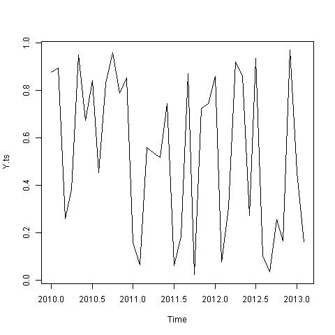
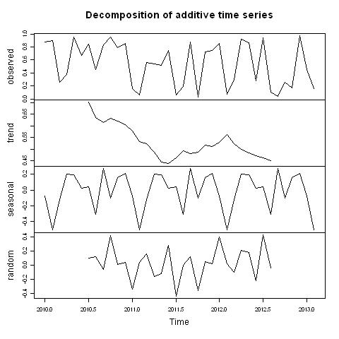
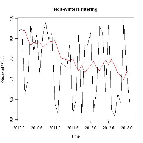
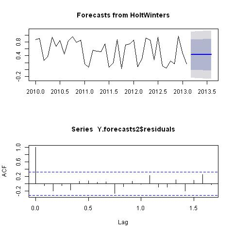
Y.ts <- ts(Y, frequency=12, start=c(2010,1)) #1: store the data in a time series object Y.forecasts <- HoltWinters(Y.ts, beta=FALSE, gamma=FALSE) #2: fit a simple exponential smoothing predictive model using the "HoltWinters()" function library("forecast") #3: load the "forecast" R package Y.forecasts2 <- forecast.HoltWinters(Y.forecasts, h=6) #4: forecast up to 6 months Y.forecasts2 #5: display forecasts par(mfrow = c(2,1)) #6: 2x1 charts plot(Y.forecasts2) #7: plot the forecasts with 80%,95% prediction interval acf(Y.forecasts2$residuals, lag.max=20) #8: correlogram of the in-sample forecast errors for lags 1-20