AutoRegressive Integrated Moving Average (ARIMA) Models

Differencing Time Series

Y.ts <- ts(Y, frequency=12, start=c(2010,1)) #1: store the data in a time series object Y.diff1 <- diff(Y.ts, differences=1) #2: difference the time series once Y.diff2 <- diff(Y.ts, differences=1) #3: difference the time series twice par(mfrow = c(2,1)) #4: 2x1 charts plot(Y.diff1) #5: plot the differencing plot(Y.diff2) #6: plot the differencing

ARIMA

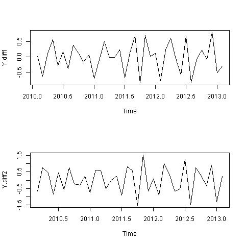
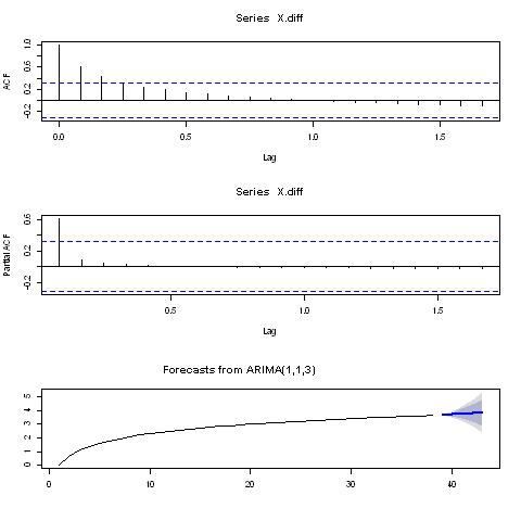
X.ts <- ts(X, frequency=12, start=c(2010,1)) #1: store the data in a time series object X.diff <- diff(X.ts, differences=1) #2: assuming not stationary then we need differencing par(mfrow = c(3,1)) #3: 3x1 charts acf(X.diff, lag.max=20) #4: correlogram for lags 1-20 to find q pacf(X.diff, lag.max=20) #5: partial correlogram for lags 1-20 to find p library("forecast") #6: load the "forecast" R package #X.arima <- auto.arima(X) #7: find an appropriate ARIMA model X.arima <- arima(X, order=c(1,1,3)) #7: use ARIMA(p,d,q) where p=1,d=1,q=3 X.arima #8: display ARIMA model X.forecasts <- forecast.Arima(X.arima, h=5) #9: forecast up to the next 5 period plot.forecast(X.forecasts) #10: plot forecast